SWOT Simulator for Ocean Science¶

Clement Ubelmann, Lucile Gaultier and Lee-Lueng Fu

Jet Propulsion Laboratory, California Institute of Technology, CNES

Abstract:¶

This software simulates sea surface height (SSH) synthetic observations of the proposed SWOT mission that can be applied to an ocean general circulation model (OGCM), allowing the exploration of ideas and methods to optimize information retrieval from the SWOT Mission in the future. From OGCM SSH inputs, the software generates SWOT-like outputs on a swath along the orbit ground track, as well as outputs from a nadir altimeter. Some measurement error and noise are generated according to technical characteristics published by the SWOT project team. Not designed to directly simulate the payload instrument performance, this SWOT simulator aims at providing statistically realistic outputs for the science community with a simple software package released as an open source in Python. The software is scalable and designed to support future evolution of orbital parameters, error budget estimates from the project team and suggestions from the science community.

Simulation of the SWOT sampling over synthetic Sea Surface Height¶

From a global or regional OGCM configuration, the software generates SSH on a 120~km wide swath at typically 1~km resolution. An illustration of outputs for a global ECCO (MITgcm) configuration is shown on Fig. 1.

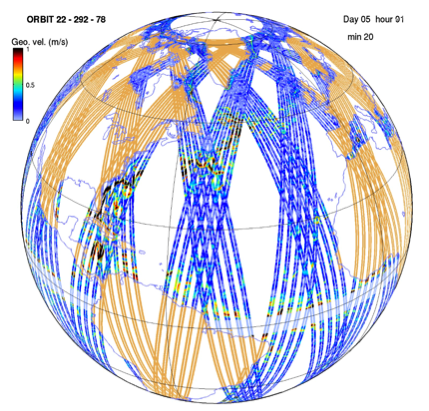
FIG. 1: 5-day worth of SWOT simulated data in a global configuration with the science orbit.¶

Proposed SWOT orbits¶

The software uses as an input the ground-tracks of the satellite orbit. The user can choose between different orbits such as the fast sampling orbit (1-day repeat), the science orbit (21-day repeat with a 10-day subcycle) and also the contingency orbit (21-day repeat with 1-day subcycle). The table below shows the characteristics of these 3 orbits:

	Repeat Cycle (days)	Repeat Cycle (Orbits)	Sub-cycles (days)	Inclination	Elevation (km)
Fast Sampling orbit	0.99349	14	N.A.	77.6	857
Science Orbit	20.8646	292	1, 10	77.6	891
Contingency orbit	20.8639	293	1	77.6	874

The ground-track coordinates corresponding to these orbits are given as input ASCII files of 3 columns (longitude, latitude, time) for one complete cycle sampled at every ~5~km. The ascending node has been arbitrarily set to zero degree of longitude, but the user can shift the orbit by any value in longitude.

Orbit files have been updated with the one provided by AVISO on september 2015 (https://www.aviso.altimetry.fr/en/missions/future-missions/swot/orbit.html). There are two additional orbit files available in the last version of the simulator. Input files are also ASCII with 3 columns (time, longitude, latitude). Orbits are provided at low resolution and are interpolated automatically by the simulator. ephem_calval_june2015_ell.txt contains the updated fast sampling orbit and ephem_science_sept2015_ell.txt the updated science orbit.

Other orbit files of the same format (time, longitude, latitude) can also be used as an input. To avoid distortions in the SWOT grid, we recommend a minimum of 10km sampling between the ground-track points of the orbit.

The SWOT swath¶

From the orbit nadir ground track the software generates a grid covering the SWOT swath over 1 cycle. In the across-swath direction, the grid is defined between 10~km and 60~km off nadir. The grid size is 2 kilometers in the along-track and across-track directions by default, but can be set at any other value (e.g. 500~m or 250~m). The longitude and latitude coordinates are referenced for each grid point, and the time coordinate (between 0 and t_cycle) is referenced in the along-track direction only. A scheme of the SWOT grid is presented on Fig. 2. The SWOT grid is stored by pass (e.g. 292 ascending passes and 292 descending passes for the science orbit). A pass is defined by an orbit starting at the lowest latitude for ascending track and at the highest latitude for descending track (+/-77.6 for the considered SWOT orbits). The first pass starts at the first lowest latitude crossing in the input file, meaning that ascending passes are odd numbers and descending passes are even numbers.

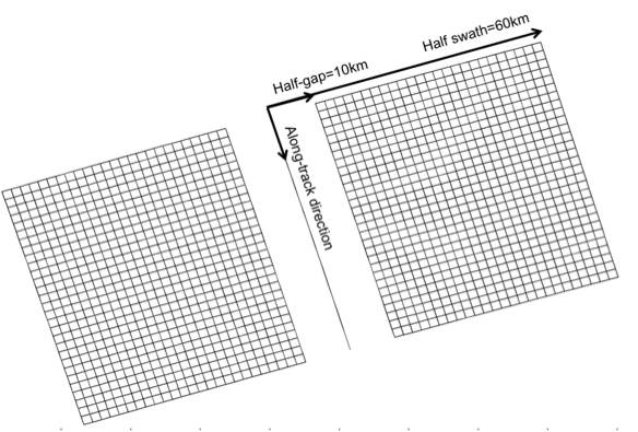
FIG. 2: scheme of the SWOT grid at 2~km resolution.¶

Interpolation of SSH on the SWOT grid and nadir track¶

SSH from the OGCM model is provided through a plugin. So far three plugins are available: One for the aviso data, with a regular time step and a regular grid, one for the LLC4320 MITGCM zar files available on CNES HAL supercomputer, and one that handles a regional hycom simulation outputs. One can build their own plugin compliant with their SSH inputs using the existing plugin as example or contact us if they need help. The SSH is interpolated on the SWOT grid and nadir track for each pass and successive cycles if the input data exceeds 1 cycle.The nadir track has the same resolution as the SWOT grid in the along-track direction, but it is possible to compute it separately with a different along track resolution. On the SWOT grid, the 2D interpolation is linear in space. No interpolation is performed in time: the SSH on the SWOT grid at a given time corresponds to the SSH of the closest time step. This avoids contaminations of the rapid signals (e.g. internal waves) if they are under-sampled in the model outputs. However, note that locally, sharp transitions of the SSH along the swath may occur if the satellite happens to be over the domain at the time of transition between two time steps. Fig. 3a shows an input SSH as an example. Fig 3b is the interpolated SSH on a 400km long segment of the SWOT grid crossing the domain.

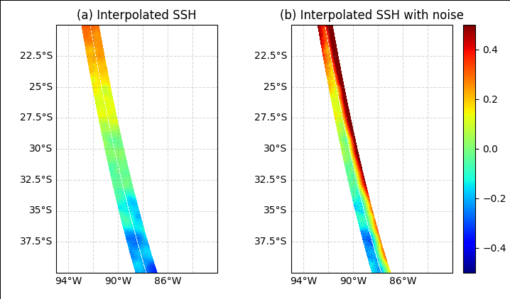
FIG. 3: SSH (in meters) produced by the MITGCM high resolution model and filtered at 1/12º.¶

a	SSH_model simulator output interpolated on the SWOT grid.
b	“Observed” SSH, which is the sum of SSH_model and a random realization of the total SWOT noise with the default parameters of the software.

Simulation of errors¶

The software generates random realizations of instrument errors and noise over the interpolated SSH, as well as simulated geophysical errors. These error simulations can be adjusted to match updates of the error budget estimation from the SWOT project team. Fig. 4 shows a realization of a SWOT error field generated by the software. It is the sum of random realizations of multiple error components described in the following. Fig. 3c shows the “observed” SSH when simulated noise is added to the interpolated SSH.

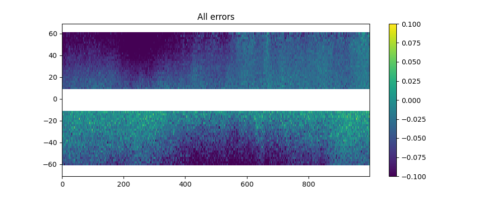
FIG. 4: Random realization of the error field (in meters). Swath coordinates are in km.¶

Instrumental errors¶

The following components of instrumental errors are implemented in the software: the KaRIN noise, the roll errors, the phase errors, the baseline dilation errors and the timing errors. Random realizations of the noise and errors are performed following the statistical descriptions of the SWOT error budget document (Esteban-Fernandez et al., 2014).

The KaRIN noise¶

The KaRIN noise is random from cell to cell, defined by a Gaussian zero-centered distribution of standard deviation inversely proportional to the square root of the cell surface. In the simulator, the KaRIN noise varies with the distance to the nadir and the Significant Wave Height (SWH) specified as a constant value between 0 and 8 meters. For a grid cell of \(1km^2\), the standard deviation of the KaRIN noise follows the curve shown on Fig. 5 with SWH varying from 0 to 8~m (Esteban-Fernandez et al., 2014). Fig. 6 shows a random realization produced by the software with \(1km^2\) grid cells and SWH=2~m.

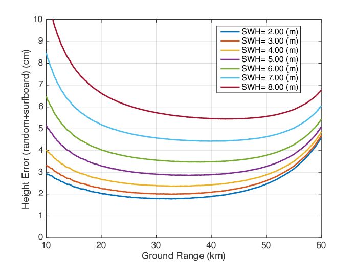
FIG. 5: The example curves of the standard deviation (cm) of the KaRIN noise as a function of cross-track distance (km).¶

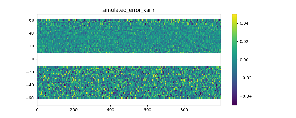
FIG. 6: Random realization of the KaRIN noise (m) following the standard deviation shown Fig. 5, with 2~km by 2~km grid cells and a varying SWH.¶

The user can define a constant value for the swh or use swh varying in time and space. In the second scenario, a plugin is necessary to read the swh and interpolate it on the SWOT grid. The plugin is similar to the one used for the SSH.

Roll knowledge and control errors¶

As detailed in Esteban-Fernandez et al., 2014, the roll error signal is the sum of two components: the roll error knowledge (also called gyro error) and the roll control errors. An estimation of the along-track power spectral density of the two roll angles is given in the input file ‘global_sim_instrument_error.nc’ from the SWOT project. It is represented on Fig. 7.

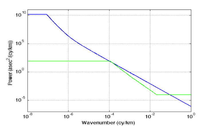
Power spectral density of the roll error

FIG. 7: Estimation of the power spectral density of the gyro error angle (blue) and the roll control error angle (green).¶

Following these spectra, random realizations of an along-track roll angle \(\theta_{roll}\) (al) are performed with uniform phase distribution. The algorithm of the random realization is described in APPENDIX A. From \(\theta_{roll}\) (al) in arcsecond unit, the power spectrum of the gyro knowledge error plus the roll control error, the total roll error h_roll (in meters) at a distance ac (in km) from the nadir is given by (see Esteban-Fernandez et al., 2014):

\[h_{roll} (al,ac)=(1+ \frac{H}{Re}) \theta_{roll} (al) \frac{\pi}{648} ac\]

where H is the altitude of the satellite and Re the earth radius. An example of realization is shown on Fig. 8.

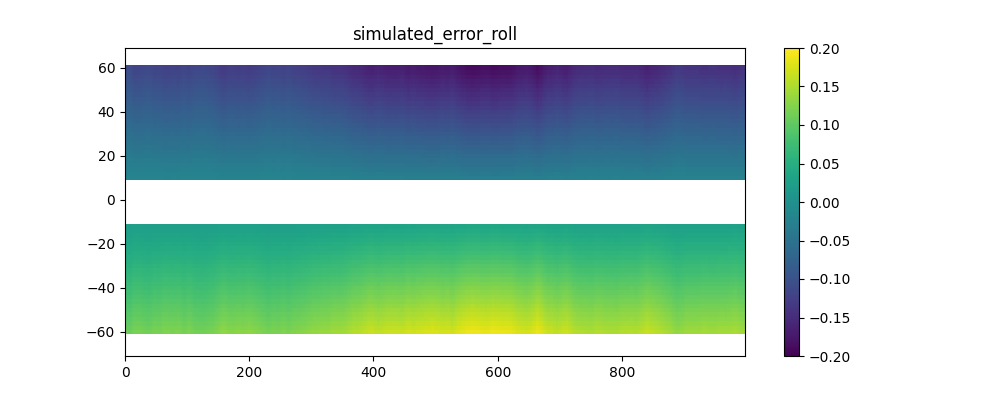
FIG. 8a: Random realization of the roll error (in m) following the power spectra of the roll angle shown Fig. 7.¶

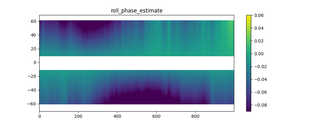
FIG. 8b: Remaining roll and phase error after cross-calibration (in m).¶

As the roll error is large, a cross-calibration has been performed for two cycles and for one year. A file is available and contains roll, phase and the correction of roll and phase usin cross-calibration algorithms. The user can use this file to simulate the roll and phase after cross-calibration.

Phase errors¶

An estimation of the along-track power spectrum of phase error is also given in the input file ‘global_sim_instrument_error.nc’. It is represented on Fig. 9.

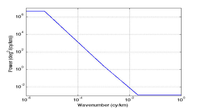
FIG. 9: Estimation of the power spectral density of the phase error¶

Following this power spectrum, random realizations of an along-track phase error \(\theta\) (al) are performed with uniform phase distribution. From \(\theta\) (al) in deg. unit, the phase error on the height \(h_{\theta}\) (in meters) at a distance ac (in km) from the nadir is given by (see Esteban-Fernandez et al., 2014):

\[h_{\theta} (al, ac) = \frac{1}{K_{Ka}B}(1+\frac{H}{Re})\theta (al) \frac{100 \pi}{18}ac\]

An independent realization of \(\theta\) is chosen for the left (ac<0) and right (ac>0) swaths. As a result, the error is decorrelated between the 2 sides (as opposed to the case of roll error), as illustrated on the random realization shown on Fig. 10.

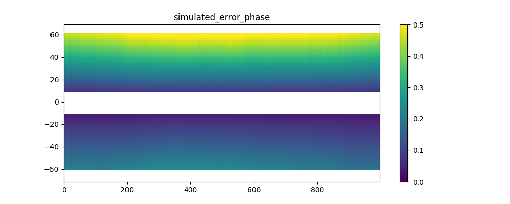
FIG. 10: Random realization of the phase error on height (in m) following the power spectra of the phase error shown Fig. 9 (with filtering of long wavelengths).¶

Like mentioned in the section regarding the roll error, the phase error is corrected using cross-calibration algorithm and available in a file that contains either two cycles or one year of data. Note that only the roll-phase-correction is available as it is not possible to correct them individually.

Baseline dilation errors¶

The baseline dilation and its resulting height measurement error is also implemented, although the errors are significantly less important than the roll and phase errors. The along-track power spectrum of the dilation \(\delta B\) is also given in the input file ‘global_sim_instrument_error.nc’. It is represented on Fig. 11.

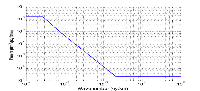
FIG. 11: Estimation of the power spectral density of the baseline dilation.¶

Following this power spectrum, random realizations of an along-track baseline dilation \(\delta B\) are performed with uniform phase distribution. From \(\delta B\) in \(\mu m\), the baseline dilation error on the height \(h_{\delta B}\) (in meters) at a distance ac (in km) from the nadir is given by the following formula (see Esteban-Fernandez et al., 2014):

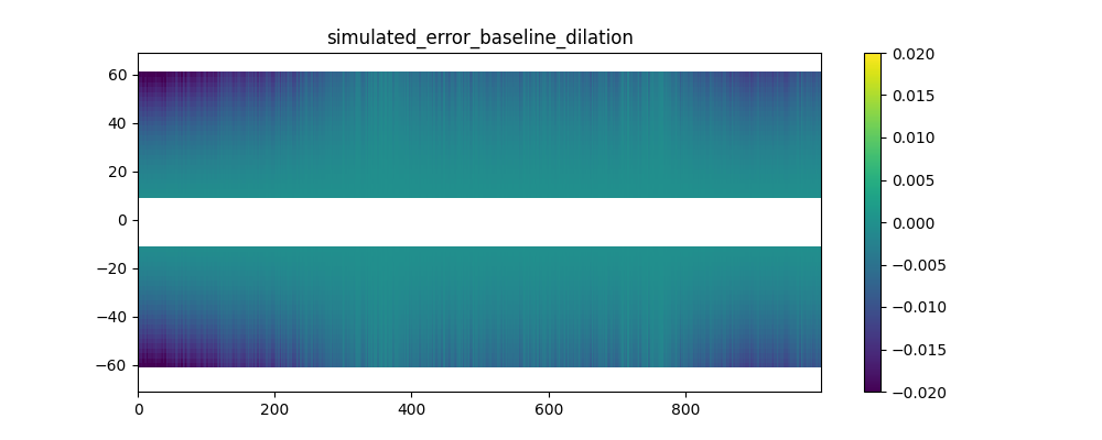
\[h_{\delta B} (al, ac) = -(1+\frac{H}{Re})\frac{\delta B(al)}{HB}ac^2\]

FIG. 12: Random realization of the baseline dilation error on height (in m) following the power spectra of the baseline dilation shown Fig. 11 (with filtering of long wavelengths).¶

Timing errors¶

The timing errors are also minor compared to roll and phase errors, but are implemented in the software. The along-track power spectrum of the timing error \(\tau\) is also given in the input file ‘global_sim_instrument_error.nc’. It is represented on Fig. 13.

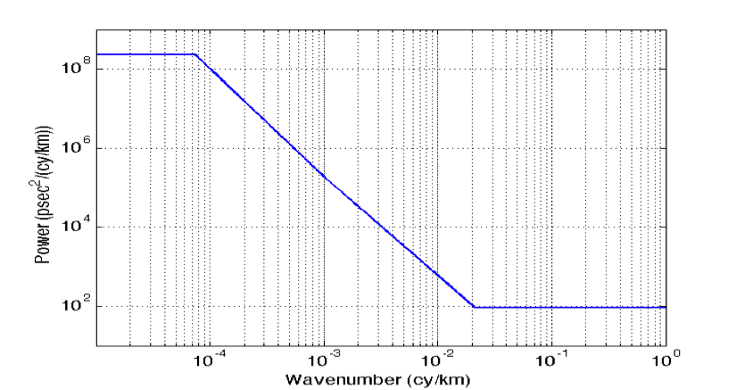
FIG. 13: Estimation of the power spectral density of the timing error¶

Following this power spectrum, random realizations of an along-track timing error \(\tau\) are performed with uniform phase distribution. From \(\tau\) (al) in pico seconds, the timing error on the height \(h_\tau\) (in meters) at a distance ac (in km) from the nadir is given by (see Esteban-Fernandez et al., 2014):

\[h_\tau (al,ac)=\frac{c}{2} \tau (al) \times 10^{-12}\]

Where c is the speed of light in m/s. The timing errors are constant in the across swath direction but independant in each part of the sath. An example is shown on Fig. 14.

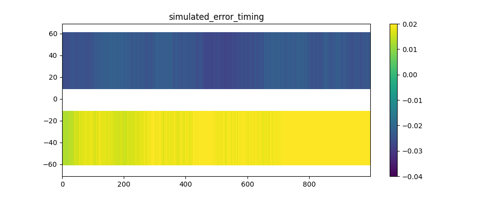
FIG. 14: Random realization of timing error on height (in m) following the power spectra of the timing error shown Fig. 13 (with filtering of long wavelengths).¶

Geophysical errors¶

So far, only the major geophysical source of error, the wet troposphere error, has been implemented in the software in a quite simple way. More realistic simulation will be hopefully implemented in the future versions.

Wet troposphere errors¶

The software simulates errors in the water vapor path delay retrieval with the option of a 1-beam radiometer configuration or a 2-beam radiometer configuration. First, a 2D random signal is generated around the swath following a 1D input spectrum, with uniform phase distribution as described in APPENDIX A. By default in the software, the 1D spectrum is the global average of estimated path delay spectrum from the AMSR-E instrument and from the JPL’s High Altitude MMIC Sounding Radiometer (Brown et al.) for the short wavelength. This spectrum is expressed by the following formula (in cm2/(cy/km)):

\[ \begin{align}\begin{aligned}S_{wet}=3.156 \times 10^{-5} f^{-8/3} \ for\ 3000km > \lambda > 100km\\S_{wet}=1.4875 \times 10^{-4} f^{-2.33} \ for\ \lambda \leq 100km\end{aligned}\end{align} \]

Fig. 15 shows a random realization of the path delay following the above spectrum. By modifying the code, the user can change the power spectrum to match the water vapor characteristics of a particular region, by using for example the global climatology provided in Ubelmann et al., 2013.

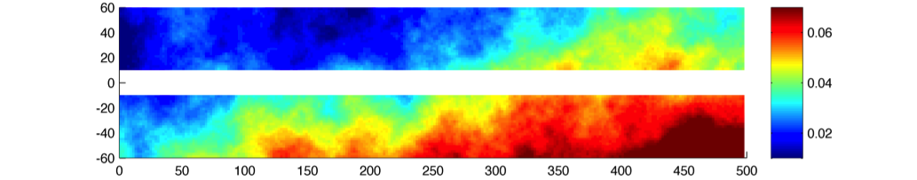
FIG. 15: Random realization of wet-tropospheric path delay without correction (in meters).¶

From the 2D random signal, the software simulates the residual error after correction for the estimated path delay from the radiometer. By default, the number of radiometer beams is set to 1. We considered that the radiometer (with 1 or 2 beams) measure the path delay averaged over a 2D Gaussian footprint with standard deviation \(\sigma_0\) (in km). \(\sigma_0\) is set at 8~km by default (corresponding to an overall 20~km diameter beam, close to the characteristic of the AMR radiometer on Jason-2), but can be modified by the user since the beam characteristics are not yet fixed by the project team. An additional radiometer instrument error is considered, given by the following characteristics (in cm2/(cy/km , see Esteban-Fernandez et al., 2014):

\[ \begin{align}\begin{aligned}S_{wet\_instr}=9.5×10^{-5} f^{-1.79} \ for\ 10^{-3} \leq f < 0.0023\\S_{wet\_instr}=0.036f^{-0.814} \ for\ 0.0023 \leq f < 0.0683\\S_{wet\_instr}=0.32\ for\ f \geq 0.0683\end{aligned}\end{align} \]

The high frequencies of instrument error (below 25km wavelength) have been filtered in the simulator. Indeed, this high-frequency signal can be easily removed since it exceeds significantly the spectral characteristics of a water vapor spectrum averaged over a 25~km diameter beam. The scheme on Fig. 16 shows how the residual error with a 1-beam or 2-beam radiometer is calculated. In the 1-beam case, the single beam measurement around the nadir plus a random realization of the radiometer instrument error is the estimate applied across the swath. In the 2-beam case, the estimation across the swath is a linear fit between the two measurements. Fig. 17 shows an example of residual error after a 1-beam and a 2-beam correction.

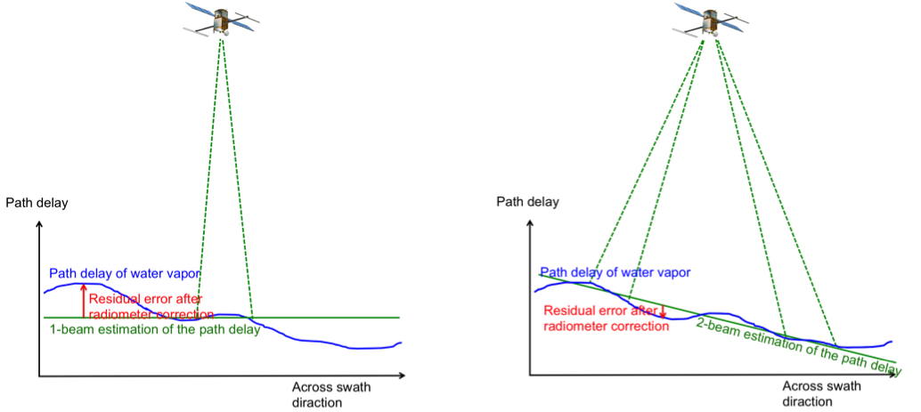
Simulation of path delay estimation and the residual error

FIG. 16: Scheme showing the simulation of the path delay estimation and the residual error for a 1-beam (left) and 2-beam (right) radiometer configuration.¶

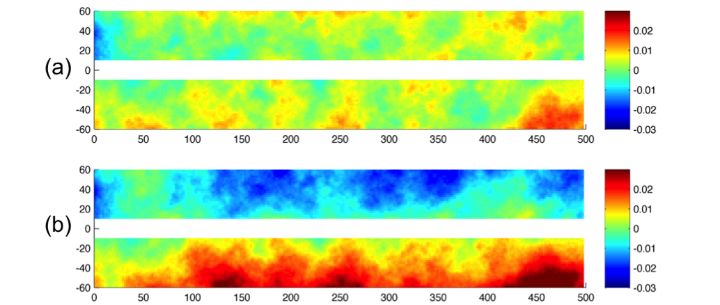
Residual error after wet-tropospheric correction using a 2-beam or 1-beam radiometer

FIG. 17: (a) Residual error after wet-tropospheric correction with the simulation of a 2-beam radiometer at 35~km away from nadir, from the simulated path delay on Fig. 15. (b) Residual error with the simulation of a 1-beam radiometer at nadir.¶

Sea state bias¶

The Sea State Bias (or Electromagnetic bias) and its estimation are not implemented in the software yet. If SWH input files are provided, SWH values are interpolated and stored on the SWOT files. SSB can be simulated offline using this output.

Other geophysical errors¶

The other geophysical errors (Dry-troposphere, Ionosphere) are not implemented in the software since they have a minor impact on the mesoscales to be observed by SWOT.

Total error budget¶

The along-track power spectra of the different error components have been computed to check the consistency with the baseline requirements. These spectra, averaged across-track between 10~km and 60~km off nadir, are represented on Fig. 18. The total error budget with a 1-beam radiometer (thick black curve) is indeed slightly below the error requirement (thick red curve).

Note that the along-track power spectrum of the KaRIN noise (dark pink thick curve) sampled on a 2~km by 2~km grid is about 6 \(cm**2/(km/cy)\), which exceeds the requirements for short wavelength. However, these requirements have been defined for wavelength exceeding 15~km in the plan (2 dimensions). Sampled at the Niquist frequency in the across swath direction (7.5~km), the noise drops down to 2 \(cm2/(km/cy)\) (thick dark pink curve).

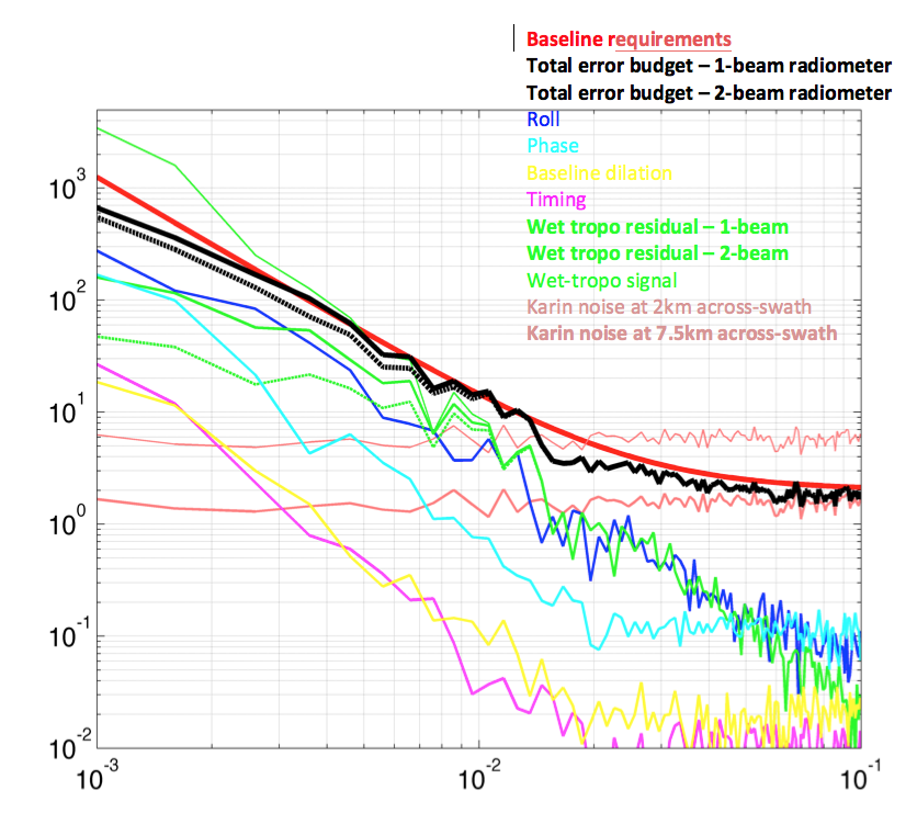
FIG. 18: Error budget in the spectral domain, computed from a random realization of the simulator. The spectral densities have been averaged across-swath between 10~km and 60~km off nadir, consistenly with the definition of the requirements.¶

Simulation of errors for the nadir altimeter¶

Two main components of the nadir altimetry error budget are simulated : the altimeter noise and residual wet-tropo errors. For the altimeter noise, the noise follow a spectrum of error consistent with global estimates from the Jason-2 altimeter. The wet tropo residual errors are generated using the simulated wet tropo signal and radiometer beam convolution described above for the KaRIN data.

The software¶

The software is written in Python3, and is mainly tested on python3.8 and 3.9. All the parameters that can be modified by the user are read in a params file (e.g. params.py) specified by the user. These parameters are written in yellow later on.

The software is divided in 6 main modules:

swot_simulator.launcher is the main program that runs the simulator.
swot_simulator.orbit_propagator generates the SWOT swath.
swot_simulator.error.generator generates all the errors on the swath, all the error modules are in the error directory.
swot_simulator.product_specification defines the format to save output in L2 SWOT-like data.
swot_simulator.settings contains parameter keys and their default values.
swot_simulator.plugins directory, which contains modules to read and interpolate model SSH and SWH.

Inputs¶

To read and interpolate SSH and SWH inputs on the SWOT grid, you have to provide your own reader as a plugin. Several readers are already available in the plugins/ssh directory for the SSH:

swot_simulator.plugins.ssh.aviso for AVISO/CMEMS data, which are on regular grid with one timestep per file
swot_simulator.plugins.ssh.hycom for HYCOM regional data
swot_simulator.plugins.ssh.mitgcm for LLC4320 MITGCM zar data (format compatible with the one available on the CNES HAL supercomputer)
swot_simulator.plugins.ssh.mitgcm_ww3 for data converted in netcdf on Datarmor IFREMER supercomputer and compatible with WW3 format.

One reader is available in the plugins/swh directory for the SWH:

swot_simulator.plugins.swh.ww3 for WW3 outputs (available on Datarmor IFREMER supercomputer)

The plugin for the ssh is specified in the ssh_plugin key, and the one for the swh in the swh_plugin key.

It is possible to generate the noise alone, without using any SSH model as ssh_pluginssh_plugin key to None.

A specific area can be specified in the area key, which will contain a list: (min_lon, min_lat, max_lon, max_lat). Default value is None and equivalent to the extend of the model.

Generation of the SWOT grid¶

The SWOT grid is generated in the swot_simulator.orbit_propagator module. The path to the orbit file is mentioned here: ephemeris, and contains longitude, latitude and the corresponding time for each point of the orbit (see section Proposed SWOT orbits for more details on the provided orbit). If different, the order of columns can be specified in ephemeris_col, default is [1, 2, 0]. The orbit is interpolated at the along track resolution specified by the user (in delta_al) and the swath is computed at each points of the orbit with an across track resolution specified by the user (in delta_ac). The width of the swath (half_swath) and the gap between the nadir and the swath (half_gap) can also be defined according to Fig. 2. The generation of the SWOT grid can be made on the whole region of the model (area = None) or on a subdomain (area = [lon_min, lat_min, lon_max, lat_max]).

Sampled SSH and error fields¶

At each pass, for each cycle, an output netcdf file containing the SSH interpolated from the model (if ssh_plugin is not set to None) and the different errors are created. The naming and the format of the file is compliant with SWOT’s PDD (Product Description Document), set complete_product key to True to store all the variables and False to store only the one compute by the simulator. You can also select the output type product_type among 'expert', 'ssh', and 'windwave'. Default is 'expert' and details are in the corresponding xml file. The output directory is defined in working_directory key, default is the user`s root. The output file names are stored in the output directory in karin/<year> directory for SWOT and nadir/<year> directory for the nadir. The naming follows the pattern SWOT_L2_LR_Expert_[cycle]_[pass]_[starttime]_[stoptime]_DG10_01.nc. The interpolation method is specified in your SSH plugin. pangeo-pyinterp module is used in the examples.

The simulator can be used to generate nadir data and / or SWOT-like data. Set the options nadir to True for nadir and swath to True for SWOT data. At least one of these options must be set to True, which is the default value.

Computation of errors are specified as a list: noise = ['altimeter', 'baseline_dilation', 'karin', 'corrected_roll_phase', 'timing', 'wet_troposphere'] 'corrected_roll_phase' error will generate already cross-calibrated roll-phase error whereas 'roll_phase' will generate errors before cross-calibration.

A repeat length len_repeat = 2000 key defines the wavelength in km to repeat the noise and is used for all noises. The path to the file that contains instrumental errors is mentioned in error_spectrum key. It is possible to specify the seed for Randomstate in nseed. The following parameters are specific to each noise componant:

KaRIN: The file noise that contains the spectrum is available in karin_noise, a constant swh can be set swh=2 or interpolated from a model SWH specified in the plugin swh_plugin.
Roll-phase: To use already cross-calibrated roll phase, download the file from the FTP (https://ftp.odl.bzh/swot) and specify the path in the corrected_roll_phase_dataset key. So far the following files are available:
- data_sim_slope_v0.nc: One year of cross-calibrated roll-phase
- data_sim_slope_2cycles_v0.nc: Two cycles of cross-calibrated roll-phase
Wet troposphere: The number of beams used to corrected for the wet troposphere is set in nbeam variable. The beam position of each beam can be set as a list in beam_position and the gaussian footprint can be changed using sigma variable.

Nadir¶

The SWOTsimulator can be used to generate any nadir like observation. The mission ephemeris should be provided as explained in Generation of the SWOT grid section. The corresponding cycle_duration and height value should be specified. Default values are for the SWOT mission:

cycle_duration=20.86455 days
height=891000 m

Getting started¶

To run the simulator:

swot_simulator --first-date '<year>-<month>-<day>T00:00:00' --last-date \
  '<year>-<month>-<day>T00:00:00' --threads-per-worker <nproc> \
  <parameter_file>

Example:

swot_simulator --first-date '2019-08-02T12:00:00' --last-date \
  '2019-08-06T00:00:00' --threads-per-worker 3  params_aviso.py

You can activate the debug mode by using –debug option in the command line.

Example of Params.txt for SWOT-like data¶

import os
import swot_simulator.plugins.ssh
import swot_simulator.plugins.swh

# Geographical area to simulate defined by the minimum and maximum corner
# point :lon_min, lat_min, lon_max, lat_max
#
# Default: None equivalent to the area covering the Earth: -180, -90, 180, 90
area = [0, -60, 20, -50]

# Distance, in km, between two points along track direction.
delta_al = 2.0

# Distance, in km, between two points across track direction.
delta_ac = 2.0

# Ephemeris file to read containing the satellite's orbit.
ephemeris = os.path.join("data_swot", "ephem_science_sept2015_ell.txt")

# Index of columns to read in the ephemeris file containing, respectively,
# longitude in degrees, latitude in degrees and the number of seconds elapsed
# since the start of the orbit.
# Default: 1, 2, 0
ephemeris_cols = [1, 2, 0]

# If true, the generated netCDF file will be the complete product compliant
# with SWOT's Product Description Document (PDD), otherwise only the calculated
# variables will be written to the netCDF file.
complete_product = True

# Distance, in km, between the nadir and the center of the first pixel of the
# swath
half_gap = 2.0

# Distance, in km, between the nadir and the center of the last pixel of the
# swath
half_swath = 70.0

# Limits of SWOT swath requirements. Measurements outside the span will be set
# with fill values.
requirement_bounds = [10, 60]

# The next two parameters (cycle_duration and height) can be read from the
# ephemeris file if it includes these values in comments. The ephemeris
# delivered with this software contain this type of declaration

# Duration of a cycle.
# #cycle_duration=

# Satellite altitude (m)
# #height=

# True to generate Nadir products
nadir = True

# True to generate swath products
swath = True

# The plug-in handling the SSH interpolation under the satellite swath.
ssh_plugin = swot_simulator.plugins.ssh.AVISO(
    "/mnt/data/data_model/cmems_nrt_008_046")

# Orbit shift in longitude (degrees)
# #shift_lon=

# Orbit shift in time (seconds)
# #shift_time=

# The working directory. By default, files are generated in the user's root
# directory.
working_directory = '/mnt/data/test_swot'

# Generation of measurement noise.

#############################
##   ERROR PARAMETERS      ##
#############################
# The calculation of roll errors can be simulated, option "roll_phase", or
# interpolated, option "corrected_roll_phase", from the dataset specified by
# the option "roll_phase_dataset". Therefore, these two options are
# mutually exclusive. In other words, if the "roll_phase" option is present,
# the "corrected_roll_phase" option must be omitted, and vice versa.
noise = [
    'altimeter',
    'baseline_dilation',
    'karin',
    'corrected_roll_phase',
    # 'roll_phase',
    'timing',
    'wet_troposphere',
]

# repeat length
len_repeat = 20000

# ---- Karin noise
# KaRIN file containing spectrum for several SWH:
karin_noise = os.path.join('data_swot', 'karin_noise_v2.nc')

# SWH for the region:
#        if swh greater than 7 m, swh is set to 7
swh = 2

# SWH plugin to interpolate model SWH on the SWOT grid:
swh_plugin = swot_simulator.plugins.ssh.WW3("/mnt/data/data_model/ww3")

# Number of km of random coefficients for KaRIN noise (recommended nrandkarin=1000):
nrand_karin = 1000

# --- Other instrumental and atmospheric noise
# File containing spectrum of instrument error:
error_spectrum = os.path.join('data_swot', 'global_sim_instrument_error.nc')

# Seed for RandomState. Must be convertible to 32 bit unsigned integers.
nseed = 0

# Roll-phase simulation of correction file
corrected_roll_phase_dataset = os.path.join('data_swot',
                                            'data_sim_slope_2cycles_v0.nc')

# Beam print size (in km):
#        Gaussian footprint of sigma km
sigma = 8.

# Number of beam used to correct wet_tropo signal (1, 2 or 12 for both):
nbeam = 2

# ------ Beam position if there are 2 beams (in km from nadir):
beam_position = [-35, 35]

References:¶

Esteban-Fernandez, D. SWOT Project Mission Performance and error budget” document, 2014 (JPL D-79084)

Ubelmann, C., Fu, L-L., Brown, S. Peral, E. and Esteban-Fernandez, D. 2014: The Effect of Atmospheric Water Vapor Content on the Performance of Future Wide-Swath Ocean Altimetry Measurement. J. Atmos. Oceanic Technol., 31, 1446–1454.

Gaultier, L., C. Ubelmann, and L-L. Fu, 2016: The challenge of using future SWOT data for oceanic field reconstruction, J. Ocean. Atm. Tech., 33, 119-126, DOI: 10.1175/JTECH-D-15-0160.1