Geophysical errors

So far, only the major geophysical source of error, the wet troposphere error, has been implemented in the software in a quite simple way. More realistic simulation will be hopefully implemented in the future versions.

Wet troposphere errors

The software simulates errors in the water vapor path delay retrieval with the option of a 1-beam radiometer configuration or a 2-beam radiometer configuration. First, a 2D random signal is generated around the swath following a 1D input spectrum, with uniform phase distribution as described in APPENDIX A. By default in the software, the 1D spectrum is the global average of estimated path delay spectrum from the AMSR-E instrument and from the JPL’s High Altitude MMIC Sounding Radiometer (Brown et al.) for the short wavelength. This spectrum is expressed by the following formula (in cm2/(cy/km)):

\[ \begin{align}\begin{aligned}S_{wet}=3.156 \times 10^{-5} f^{-8/3} \ for\ 3000 km > \lambda > 100 km\\S_{wet}=1.4875 \times 10^{-4} f^{-2.33} \ for\ \lambda \leq 100 km\end{aligned}\end{align} \]

Fig. 15 shows a random realization of the path delay following the above spectrum. By modifying the code, the user can change the power spectrum to match the water vapor characteristics of a particular region, by using for example the global climatology provided in Ubelmann et al., 2013.

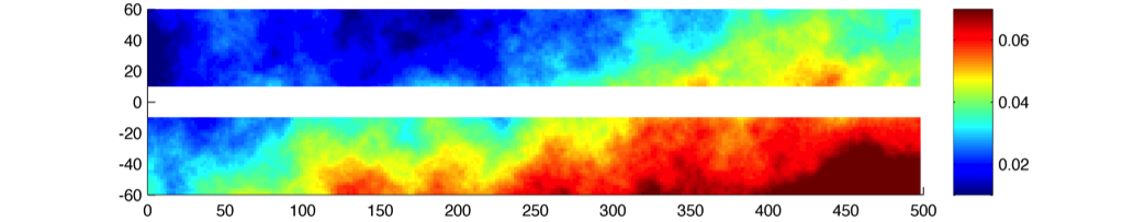
FIG. 15: Random realization of wet-tropospheric path delay without correction (in meters).

From the 2D random signal, the software simulates the residual error after correction for the estimated path delay from the radiometer. By default, the number of radiometer beams is set to 1. We considered that the radiometer (with 1 or 2 beams) measure the path delay averaged over a 2D Gaussian footprint with standard deviation \(\sigma_0\) (in km). \(\sigma_0\) is set at 8~km by default (corresponding to an overall 20~km diameter beam, close to the characteristic of the AMR radiometer on Jason-2), but can be modified by the user since the beam characteristics are not yet fixed by the project team. An additional radiometer instrument error is considered, given by the following characteristics (in cm2/(cy/km , see Esteban-Fernandez et al., 2014):

\[ \begin{align}\begin{aligned}S_{wet\_instr}=9.5×10^{-5} f^{-1.79} \ for\ 10^{-3} \leq f < 0.0023\\S_{wet\_instr}=0.036f^{-0.814} \ for\ 0.0023 \leq f < 0.0683\\S_{wet\_instr}=0.32\ for\ f \geq 0.0683\end{aligned}\end{align} \]

The high frequencies of the instrument error (below 25 km wavelength) have been filtered in the simulator. Indeed, this high-frequency signal can be easily removed since it exceeds significantly the spectral characteristics of a water vapor spectrum averaged over a 25~km diameter beam. The scheme in Fig. 16 shows how the residual error with a 1-beam or 2-beam radiometer is calculated. In the 1-beam case, the single beam measurement around the nadir plus a random realization of the radiometer instrument error is the estimate applied across the swath. In the 2-beam case, the estimation across the swath is a linear fit between the two measurements. Fig. 17 shows an example of residual error after a 1-beam and a 2-beam correction.

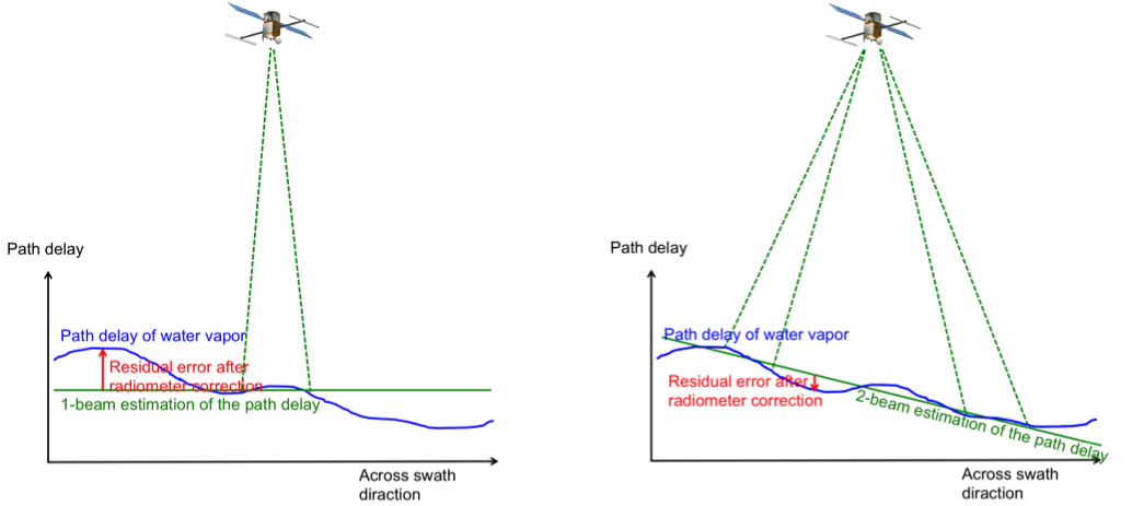
FIG. 16: Scheme showing the simulation of the path delay estimation and the residual error for a 1-beam (left) and 2-beam (right) radiometer configuration.

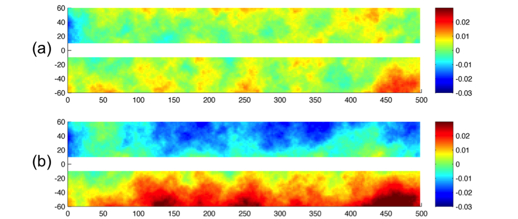
FIG. 17: (a) Residual error after wet-tropospheric correction with the simulation of a 2-beam radiometer at 35~km away from nadir, from the simulated path delay on Fig. 15.
(b) Residual error with the simulation of a 1-beam radiometer at nadir.

Sea state bias

The Sea State Bias (or Electromagnetic bias) and its estimation are not implemented in the software yet. If SWH input files are provided, SWH values are interpolated and stored on the SWOT files. SSB can be simulated offline using this output.

Other geophysical errors

The other geophysical errors (Dry-troposphere, ionosphere) are not implemented in the software since they have a minor impact on the meso-scales to be observed by SWOT.